V-plotter math

The most important thing to deal with in v-plotter software is the coordinate transformation. Descartes coordinates must be converted to the coordinate system of the plotter. In the most simple case, when the strings meet at one point of the carriage, this is a trivial task, straightforward application of the Pythagoras theorem.

However, such a simple design comes with a price as the carriage becomes unstable. And this happens when one tries to stabilize it without adjusting the coordinate transformation:

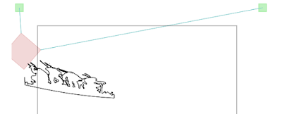
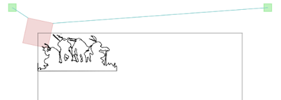
The reason for the distorted image lies in the rotation of the carriage that must be compensated to get the proper drawings:

In the following I explain the method I came up with to compensate the rotation. This method is integrated with my v-plotter step generator, and there is also a prototype Java application available for educational purposes.

V-Plotter carriage

Let us suppose that we have a v-plotter and the pen is in the center of the mass of its carriage. The task is to answer, given the \(C(x,y)\) coordinate, one of these three identical questions:

the rotation angle \((\gamma)\) of the box
the coordinates of the \(A\) and \(B\) points
the lengths of the strings.

The idea is that for any given \(C(x,y)\) there must be exactly one \(\gamma\) that nature chooses, the angle where the sum of torques acting on the carriage is zero.

First, for a given \(C(x,y)\) and \(\gamma\), we need to calculate the torques exerted on the carriage by the two strings. The algorithm consist of the following steps:

V-Plotter carriage rotation

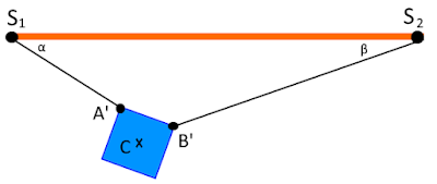
Given \(C(x,y)\) and the dimensions of the carriage, calculate the \(A\) and \(B\) points (considering that the rotation is zero)
Rotate the carriage around \(C\) by \(\gamma\) to get \(A’\) and \(B’\)
Calculate the \(\alpha\) and \(\beta\) angles
Calculate the \(T_1\) and \(T_2\) tensions in the strings using the following formulas:

Note: For explanation, read the details at the end of the post.

\[ T_1 = \frac{F_g}{\cos \alpha \tan \beta + \sin \alpha} \qquad T_2 = T_1 \frac{\cos \alpha}{\cos \beta} \] where \(F_g = mg\), the mass of the carriage multiplied by the gravity constant.

Calculate the force vectors: \[ \vec{F_1} = \frac{\vec{S_1A’}}{\lvert\vec{S_1A’}\rvert} T_1 \qquad \vec{F_2} = \frac{\vec{S_2B’}}{\lvert\vec{S_2B’}\rvert} T_2 \]
Calculate torques. Torque is the cross product of the force vector and the level arm vector: \[ \tau_1 = \vec{A’C} \times \vec{F_1} \qquad \tau_2 = \vec{B’C} \times \vec{F_2} \]

Finally, let’s create a function that implements this algorithm and returns the sum of the torques:

\[\tau(x,y)( \gamma) = \tau_1 + \tau_2\]

As we need to find the angle where \(\tau_1 + \tau_2 = 0\), that is the carriage is in rotational equilibrium, the next step is to calculate the root of the \(\tau(x,y)\) function. This function is strictly monotone, thus Newton’s iteration can be applied with an initial guess of \(0\) degrees.

A prototype implementation can be found here, and if you are interested in the details of the tension equations, read further (and watch the lecture about the super hot tension problem):

Note: To find the tension in the strings, Newton’s second law must be solved: \[a = \frac{\sum{F}}{m}\] Or rather these: acceleration is required to be zero and the equation is split, because it is easier to solve the vertical and horizontal projections one by one: \[0 = \frac{\sum{F_x}}{m}\] \[0 = \frac{\sum{F_y}}{m}\] First, the \(x\) direction: \[0 = \frac{T_{1x}-T_{2x}}{m}\] that is \[T_{1x} = T_{2x}\tag{1}\] The \(y\) direction is only a tiny bit more complicated as the force of gravity is also must be taken into account: \[0 = \frac{-F_g+T_{1y}+T_{2y}}{m}\] which is \[F_g = T_{1y}+T_{2y}\tag{2}\] The vertical and horizontal projections of \(T_1\) and \(T_2\) are simple like this (at this point the \(\alpha\) and \(\beta\) angles are already calculated): \[ T_{1x} = T_1 \cos \alpha \tag{3} \] \[ T_{2x} = T_2 \cos \beta \tag{4} \] \[ T_{1y} = T_1 \sin \alpha \tag{5} \] \[ T_{2y} = T_2 \sin \beta \tag{6} \] Now substitute \((3)\) and \((4)\) into \((1)\): \[T_1 \cos \alpha = T_2 \cos \beta\] From that: \[T_1 = T_2 \frac{\cos \beta}{\cos \alpha}\tag{7}\] Combining \((5)\) and \((7)\), \(T_{1y}\) can be expressed now as: \[T_{1y} = T_2 \cos \beta \tan \alpha\tag{8}\] Substitute \((6)\) and \((8)\) into \((2)\): \[F_g = T_{2}(\cos \beta \tan \alpha + \sin beta)\tag{9}\] The final equations can be derived directly from \((7)\) and \((9)\).